OpenCL Fast Fourier Transform

Fast Fourier Transform algorithms

Introduction

The Fast Fourier Transform is a family of algorithms computing the Discrete Fourier Transform (DFT) in time O(N.log(N)). The most commonly used FFT algorithms use a divide-and-conquer approach similar to the algorithm of Cooley and Tukey (1965). The Wikipedia FFT page is a good starting point for the interested reader.

The computation of a DFT of length N is done by splitting the input sequence into a fixed small number of smaller subsequences, compute their DFT, and assemble the outputs to build the final sequence. Providing the split and assembly steps have linear cost, the complexity of the algorithm will be O(N.log(N)).

One of the simplest subdivision is to take the sub-sequence xe with even indices 0,2,4,...,N-2, and xo with odd indices 1,3,...,N-1, supposing N is even. Compute the DFT of each sub-sequence, ye=DFT_N/2(θ²,xe) and yo=DFT_N/2(θ²,xo). Then we can build y=DFT_N(θ,x) as follows:
y_k = ye_k + θ^k yo_k, and
y_k+N/2 = ye_k - θ^k yo_k, for k=0..N/2-1.

More details on subdivisions

In this section, we enter into more details about the various subdivision schemes used in FFT, known as decimation in frequency (DIF), and decimation in time (DIT). Both actually refer to the same algorithm.

Consider a sequence x=(x₀,x₁,...,x_N-1) of length N, and a factorization N=P*Q. We denote the DFT of x of length N by DFT_N(x) or DFT_N(x₀,x₁,...,x_N-1). Let θ=e^-2*i*Π/N, y=DFT_N(x) is by definition:

y_k = θ^0.k.x₀ + θ^1.k.x₁ + θ^2.k.x₂ + ... (N terms).

We consider the P subsequences of x with length Q defined by elements with the same index modulo P:
x[u]=(x_u,x_u+P,x_u+2.P,...,x_u+(Q-1).P) with u=0..P-1.

Highlighting the terms of x[u] in y_k, we get:
y_k = ... + θ^u.k.x_u + ... + θ^(u+P).k.x_u+P + ... + θ^(u+2.P).k.x_u+2.P + ..., or
y_k = Σ_u θ^u.k (x_u + θ^P.k.x_u+P + θ^2.P.k.x_u+2.P + ...), and finally
y_k = Σ_u θ^u.k DFT_Q(x[u])_k, where element k of a DFT of length Q is taken modulo Q.

Let's group together the P values of k using the same element v of y[u]=DFT_Q(x[u]), by expressing k as k=v+Q.j, with v=0..Q-1 and j=0..P-1:
y_v+Q.j = Σ_u θ^u.(v+Q.j) y[u]_v, or
y_v+Q.j = Σ_u θ^Q.u.j (θ^u.v y[u]_v), and finally
y_v+Q.j = DFT_P(θ^0.v y[0]_v,θ^1.v y[1]_v,...,θ^(P-1).v y[P-1]_v)_j.

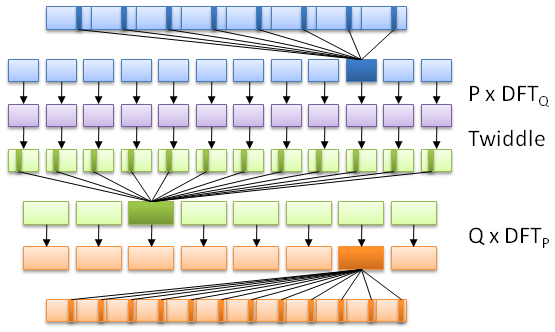
We have shown that the DFT_N can be computed by:
- compute P×DFT_Q,
- scale all the N resulting values by the "twiddle factors" θ^u.v,
- compute Q×DFT_P.

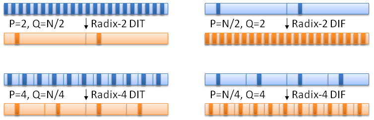
This algorithm is called either radix-P decimation in time (DIT), or radix-Q decimation in frequency (DIF). Usually, the name is chosen according to the smallest value between P and Q. A radix-2 DIT algorithm corresponds to P=2 and Q=N/2; it starts with 2 DFT_N/2. A radix-2 DIF algorithm corresponds to P=N/2 and Q=2; it starts with N/2 DFT₂.

In the next page, Reference implementations, we show how the performance of the reference implementations is measured.