OpenCL Multiprecision
Eric Bainville - Jan 2010The Schönhage-Strassen Algorithm (SSA)
Combination patterns
For more details on the SSA, refer to the Wikipedia page, and the paper A GMP-based Implementation of Schönhage-Strassen's Large Integer Multiplication Algorithm by Pierrick Gaudry, Alexander Kruppa, and Paul Zimmermann.
The SSA uses a Discrete Fourier Transform, but instead of complex numbers, the values are integers modulo 2m+1 or 2m-1 for some m. The algorithm is applied recursively, with smaller and smaller values of m.
The interesting point about SSA is that ω, the n-th root of 1, can be chosen (under certain conditions) to be a power of B. In this case the basic operation, a product by ωi, reduces to a fast shift+add combination.
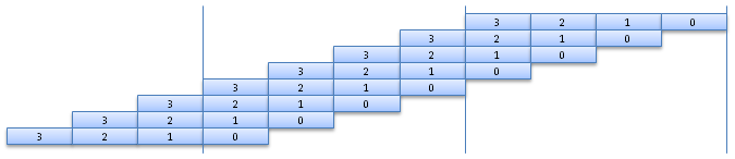
This is illustrated in the following example. Here we have a polynomial P with 8 coefficients a, b, ..., h, defined by P(X)=a.X0+b.X1+c.X2+...+h.X7. Each coefficient C (a, b,...) is written on 4 "digits": C=C0+B*C1+B2*C2+B3*C3, and we want to compute the 8 values P(B0), P(B1), ..., P(B7) modulo B4+1.
The stacks represent a sum of the 8 coefficients. The first row is for a, the second for b, etc. In the figure below, the stack represents P(B1)=a.B0+b.B1+c.B2+...+h.B7:
Now, since B4=-1, we can wrap the coefficients, changing sign each time a B4 factor is removed. The P(B1) stack is then equivalently rewritten:
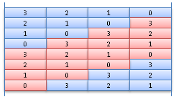
The 8 values P(Bi) can be represented by similar stacks, as shown here:
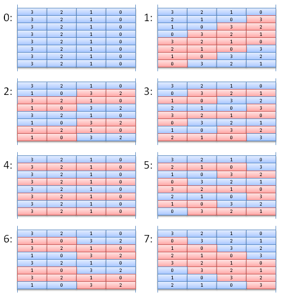
As seen in the previous page, the usual FFT algorithm recursively computes the values for even and odd numbered sub-sequences.
Example
As a more detailed complement to the Wikipedia page, let's see how we can compute the square of a 12-digit decimal number using SSA.
X = 383 886 777 915
We will represent X by a polynomial with N=8 coefficients modulo 108+1. Coefficients are stored in base B=100 on four digits. The number X is then stored on 1/4 of the 32 input digits. This is required to handle correctly the degree of the output polynomial, and the magnitude of its coefficients. The coefficients of the input polynomial P are then:
P0 = +000 +000 +009 +015
P1 = +000 +000 +007 +077
P2 = +000 +000 +008 +086
P3 = +000 +000 +003 +083
P4 = +000 +000 +000 +000
P5 = +000 +000 +000 +000
P6 = +000 +000 +000 +000
P7 = +000 +000 +000 +000
The stacks used to compute the 8 values are given below. For each stack, we display the shifted and wrapped coefficients, raw sum, and the corresponding normalized value. All values modulo 108+1 can be normalized with coefficients in the range 0..99, except for 108, represented by +000 +000 +000 -001.
          +000 +000 +009 +015
          +000 +000 +007 +077
          +000 +000 +008 +086
          +000 +000 +003 +083
          +000 +000 +000 +000
          +000 +000 +000 +000
          +000 +000 +000 +000
          +000 +000 +000 +000
raw sum = +000 +000 +027 +261
P(B0) = +000 +000 +029 +061

          +000 +000 +009 +015
          +000 +007 +077 +000
          +008 +086 +000 +000
          +083 +000 +000 -003
          +000 +000 +000 +000
          +000 +000 +000 +000
          +000 +000 +000 +000
          +000 +000 +000 +000
raw sum = +091 +093 +086 +012
P(B1) = +091 +093 +086 +012

          +000 +000 +009 +015
          +007 +077 +000 +000
          +000 +000 -008 -086
          -003 -083 +000 +000
          +000 +000 +000 +000
          +000 +000 +000 +000
          +000 +000 +000 +000
          +000 +000 +000 +000
raw sum = +004 -006 +001 -071
P(B2) = +003 +094 +000 +029

          +000 +000 +009 +015
          +077 +000 +000 -007
          -008 -086 +000 +000
          +000 +003 +083 +000
          +000 +000 +000 +000
          +000 +000 +000 +000
          +000 +000 +000 +000
          +000 +000 +000 +000
raw sum = +069 -083 +092 +008
P(B3) = +068 +017 +092 +008
|
          +000 +000 +009 +015
          +000 +000 -007 -077
          +000 +000 +008 +086
          +000 +000 -003 -083
          +000 +000 +000 +000
          +000 +000 +000 +000
          +000 +000 +000 +000
          +000 +000 +000 +000
raw sum = +000 +000 +007 -059
P(B4) = +000 +000 +006 +041

          +000 +000 +009 +015
          +000 -007 -077 +000
          +008 +086 +000 +000
          -083 +000 +000 +003
          +000 +000 +000 +000
          +000 +000 +000 +000
          +000 +000 +000 +000
          +000 +000 +000 +000
raw sum = -075 +079 -068 +018
P(B5) = +025 +078 +032 +019

          +000 +000 +009 +015
          -007 -077 +000 +000
          +000 +000 -008 -086
          +003 +083 +000 +000
          +000 +000 +000 +000
          +000 +000 +000 +000
          +000 +000 +000 +000
          +000 +000 +000 +000
raw sum = -004 +006 +001 -071
P(B6) = +096 +006 +000 +030

          +000 +000 +009 +015
          -077 +000 +000 +007
          -008 -086 +000 +000
          +000 -003 -083 +000
          +000 +000 +000 +000
          +000 +000 +000 +000
          +000 +000 +000 +000
          +000 +000 +000 +000
raw sum = -085 -089 -074 +022
P(B7) = +014 +010 +026 +023
|
The transformed vector Q, containing all values P(Bk) is then:
Q0 +000 +000 +029 +061
Q1 +091 +093 +086 +012
Q2 +003 +094 +000 +029
Q3 +068 +017 +092 +008
Q4 +000 +000 +006 +041
Q5 +025 +078 +032 +019
Q6 +096 +006 +000 +030
Q7 +014 +010 +026 +023
We now have to compute the squares of each of these values. In the real world, these would be numbers much smaller than the initial input, and the products would be handled by the most appropriate algorithm for this size: SSA for the largest ones, Karatsuba or Toom-Cook for the medium range, and trivial multiplication for the smallest ones.
Q20 +008 +076 +075 +021
Q21 +091 +095 +094 +062
Q22 +028 +036 +056 +003
Q23 +057 +002 +032 +021
Q24 +000 +041 +008 +081
Q25 +075 +035 +042 +018
Q26 +071 +032 +056 +008
Q27 +073 +049 +012 +090
To get the coefficients of the result, we now have to apply the inverse Fourier Transform. Up to a permutation and a constant factor, it can be done by applying exactly the same transformation to Q2. Doing this, we obtain the coefficients R. The number in parentheses gives the index of the coefficient in the non-permuted result:
R0 +006 +069 +078 +000  (0)
R1 +000 +000 +000 +000  (7)
R2 +001 +017 +035 +012  (6)
R3 +005 +042 +094 +008  (5)
R4 +011 +004 +014 +024  (4)
R5 +016 +062 +018 +072  (3)
R6 +017 +080 +008 +072  (2)
R7 +011 +037 +052 +080  (1)
The last step is to assemble the result, using 3 digits per coefficient. Each coefficient must first be divided by N=8:
+006 +069 +078 +000 =>                         837 225
+011 +037 +052 +080 =>                   1 421 910
+017 +080 +008 +072 =>               2 225 109
+016 +062 +018 +072 =>           2 077 734
+011 +004 +014 +024 =>       1 380 178
+005 +042 +094 +008 =>     678 676
+001 +017 +035 +012 => 146 689
+006 +069 +078 +000 =>   0
X^2 =                  147 369 058 257 960 531 747 225
Recursive evaluation
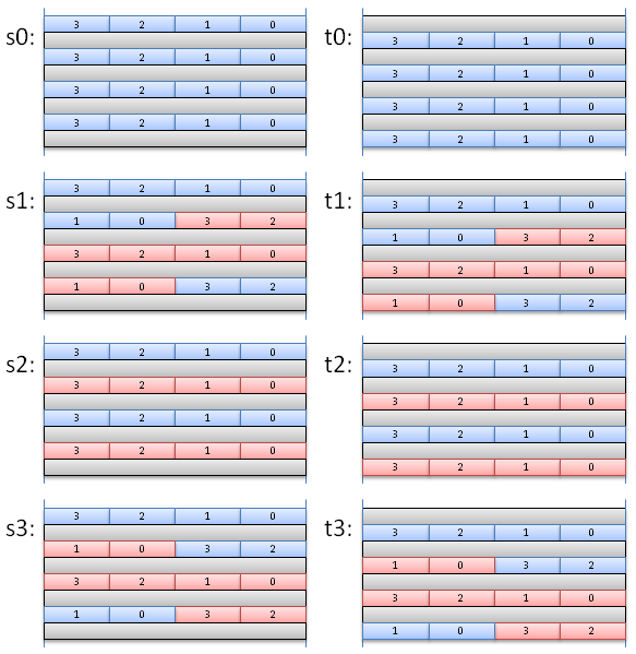
The basic operation of the recursive algorithm takes two rows x and y and combines them into x+ωk.i.y and x-ωk.i.y. Except for the initial step, requiring a permutation, it can be done "in-place" in memory, replacing the two input rows with the outputs. This basic operation is called a "butterfly". There are log2(N) levels of recursion, and each level requires N/2 butterflies.
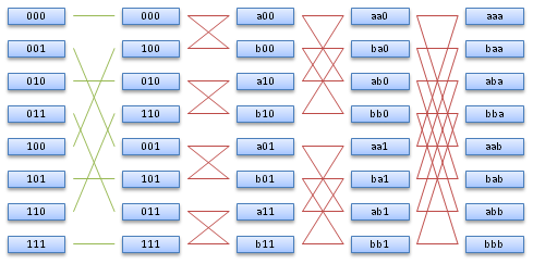
In our example, we would compute the following:
Input values   reverse binary permutation
+000 +000 +009 +015   ---------   +000 +000 +009 +015
+000 +000 +007 +077   -. .-----   +000 +000 +000 +000
+000 +000 +008 +086   --|------   +000 +000 +008 +086
+000 +000 +003 +083   --|--. .-   +000 +000 +000 +000
+000 +000 +000 +000   -' '--|--   +000 +000 +007 +077
+000 +000 +000 +000   ------|--   +000 +000 +000 +000
+000 +000 +000 +000   -----' '-   +000 +000 +003 +083
+000 +000 +000 +000   ---------   +000 +000 +000 +000

                   Combine 1
+000 +000 +009 +015   -..-  +000 +000 +009 +015
+000 +000 +000 +000   -''-  +000 +000 +009 +015
+000 +000 +008 +086   -..-  +000 +000 +008 +086
+000 +000 +000 +000   -''-  +000 +000 +008 +086
+000 +000 +007 +077   -..-  +000 +000 +007 +077
+000 +000 +000 +000   -''-  +000 +000 +007 +077
+000 +000 +003 +083   -..-  +000 +000 +003 +083
+000 +000 +000 +000   -''-  +000 +000 +003 +083


                     Combine 2                     Combine 3
+000 +000 +009 +015  -. .-      +000 +000 +017 +101 -.   .- +000 +000 +027 +261
+000 +000 +009 +015    X  -. .- +008 +086 +009 +015   \ /   +091 +093 +086 +012
+000 +000 +008 +086  -' '-  X   +000 +000 +001 -071    X    +004 -006 +001 -071
+000 +000 +008 +086       -' '- -008 -086 +009 -015   / \   +069 -083 +092 +008
+000 +000 +007 +077  -. .-      +000 +000 +010 +160 -'   '- +000 +000 +007 -059
+000 +000 +007 +077    X  -. .- +003 +083 +007 +077    .    -075 +079 -068 +018
+000 +000 +003 +083  -' '-  X   +000 +000 +004 -006    .    -004 +006 +001 -071
+000 +000 +003 +083       -' '- -003 -083 +007 +077    .    -085 -089 -074 +022
In the next page, we will experiment implementations of the SSA in OpenCL.
| OpenCL Multiprecision : Multiplication Algorithms | Top of Page | OpenCL Multiprecision : OpenCL SSA I |